15. Platform Operations, Observability & SRE
Learning objective: move from building Databricks workloads to operating an enterprise data platform reliably. Learn how to observe every layer, define service objectives, detect degradation before business users do, investigate failures, manage incidents, forecast capacity, control operational cost and continuously improve reliability.
A Databricks architect is not finished when a pipeline runs successfully.
The architect must prove that the platform can keep running, meet business deadlines, detect failures, recover predictably, explain its behavior and control its cost.
This chapter is the operational engineering layer of the masterclass. It builds on Lakeflow Jobs, Structured Streaming, Lakeflow Connect, Unity Catalog, security hardening and CI/CD. It explains how to operate those capabilities as one production platform.
Official starting points:
- https://docs.databricks.com/aws/en/lakehouse-architecture/deployment-guide/observability
- https://docs.databricks.com/aws/en/data-engineering/observability-best-practices
1. The shift from development to operations
A development mindset asks:
Does the job run?
An operations mindset asks:
- Does it finish before the business deadline?
- Is its output complete and correct?
- Is the data fresh enough for the consumer?
- Is its performance stable?
- Can we detect a failure quickly?
- Can the on-call engineer diagnose it?
- Can we recover without corrupting downstream data?
- Is the service operating within its cost budget?
A green execution is only one signal.
A pipeline can succeed technically while delivering stale, incomplete or incorrect data.
2. What is platform operations?
Platform operations is the discipline of keeping the Databricks environment and its workloads available, secure, performant, observable and economically sustainable.
| Layer | Operational responsibility |
|---|---|
| Account and workspace | Availability, identity, configuration, access |
| Compute | Capacity, utilization, startup, scaling, failures |
| Data engineering | Job and pipeline completion, correctness, freshness |
| Streaming | Throughput, lag, state, checkpoint health |
| SQL and BI | Query latency, queuing, concurrency, warehouse availability |
| Governance | Access, lineage, audit and policy health |
| Integration | Source connectivity, API limits, CDC capture |
| Cost | Usage attribution, budgets, efficiency |
| People and process | Ownership, on-call, incident response and change control |
An enterprise operating model needs visibility into all of these layers.
3. Animated operations architecture
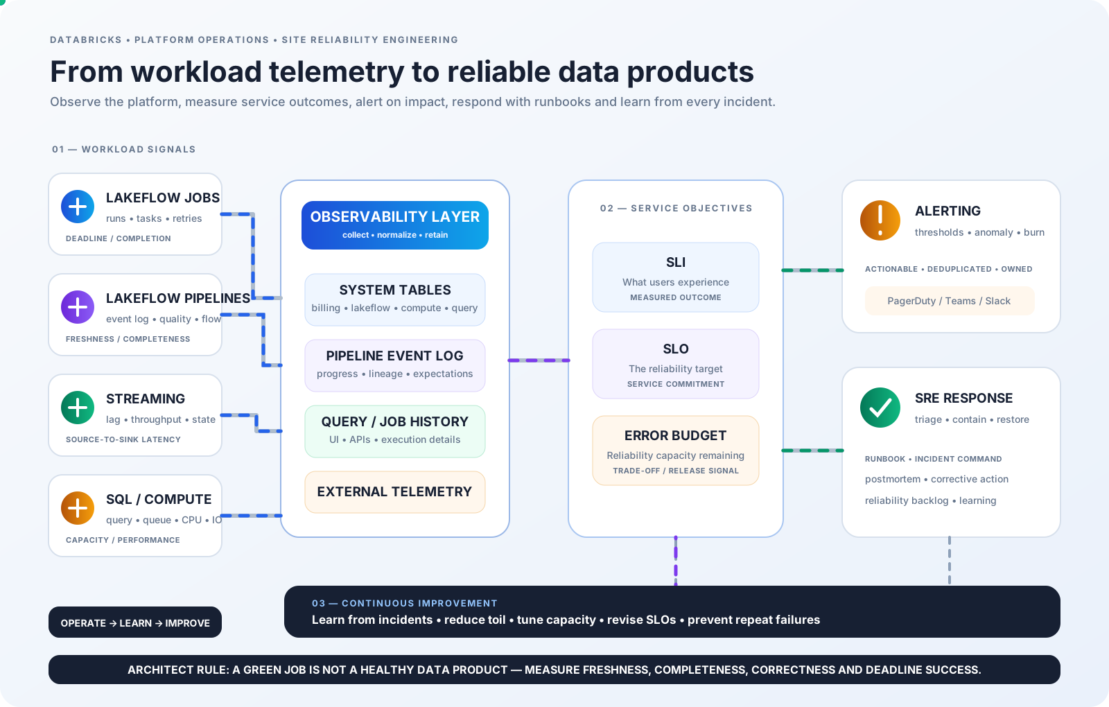
The diagram connects workload telemetry to Databricks-native observability, system tables and pipeline event logs. Those signals become service-level indicators, objectives and error budgets, which drive actionable alerts, incident response and continuous improvement.
The architect's responsibility is to connect technical signals to business impact.
4. Monitoring, observability and SRE are different
These terms are related but not interchangeable.
Monitoring
Monitoring tells you whether known conditions are healthy.
Examples:
- job failed;
- CPU utilization exceeded a threshold;
- a warehouse has queued queries;
- pipeline update duration increased.
Observability
Observability helps you investigate why a system behaves the way it does.
It combines:
- metrics;
- logs;
- traces or execution details;
- events;
- context such as identity, release, workload and dependency.
Site Reliability Engineering
SRE applies engineering practices to reliability and operations.
It introduces:
- service-level indicators;
- service-level objectives;
- error budgets;
- incident response;
- automation and toil reduction;
- capacity and performance planning;
- blameless postmortems.
A mature team needs all three.
5. The four golden signals
A practical starting model for service health is the four golden signals.
| Signal | Question | Databricks examples |
|---|---|---|
| Latency | How long does the operation take? | Job completion time, query latency, data freshness |
| Traffic | How much work is arriving? | Rows, files, events, queries, concurrent users |
| Errors | How often does work fail? | Failed runs, rejected records, query failures |
| Saturation | How close is the resource to its limit? | CPU, memory, queueing, backlog, warehouse capacity |
Do not monitor only CPU and memory.
A streaming platform can be saturated through state growth or source backlog even when CPU appears moderate.
A SQL warehouse can be saturated by concurrency and queueing even when its underlying compute appears healthy.
6. Define the service before defining the dashboard
A dashboard should begin with a service definition.
Example:
Service: Enterprise Finance Data Product
Consumers: Finance analysts, planning application and regulatory reporting
Critical outputs:
- daily actuals;
- cost center balances;
- procurement commitments;
- month-end reporting aggregates.
Business deadline: 06:00 local business time.
Freshness expectation: source data through the previous business day.
Owner: Finance Data Engineering.
Severity: Tier 1.
Now monitoring can focus on whether the service meets its business contract.
Without a service definition, teams often create dashboards full of metrics that nobody uses to make decisions.
7. SLI, SLO, SLA and OLA
These are related concepts, but they serve different purposes.
| Term | Meaning | Example |
|---|---|---|
| SLI | Service-level indicator: the measured outcome | Percentage of daily datasets ready by 06:00 |
| SLO | Service-level objective: the internal reliability target | 99.5% of scheduled daily deliveries meet the deadline |
| SLA | Service-level agreement: an external or formal commitment | Agreed availability or data-delivery commitment |
| OLA | Operational-level agreement: an internal dependency commitment | Source team provides files by 04:30 |
Architect rule
Never publish an SLA that depends on a source, network, identity or upstream team without an agreed OLA or dependency contract.
An SLO is useful even when no customer-facing SLA exists.
8. Design the right SLI for batch data
For a daily batch data product, job success alone is not a sufficient SLI.
A stronger indicator is:
SCHEDULED DELIVERY SUCCESS
=
DELIVERIES READY BEFORE DEADLINE
--------------------------------
TOTAL ELIGIBLE SCHEDULED DELIVERIES
A delivery should count as successful only when the required output is:
- available;
- complete enough;
- valid against required quality rules;
- produced before the deadline.
A job that succeeds at 06:40 when the deadline is 06:00 should not count as an on-time delivery.
Define exclusions carefully, such as an officially declared source outage.
Do not exclude failures after they occur simply to improve the reported SLI.
9. Design the right SLI for streaming
For streaming, a useful set of indicators includes:
- source-to-sink latency;
- percentage of events processed within the freshness target;
- backlog age;
- processing throughput relative to arrival rate;
- failed or quarantined event rate;
- checkpoint and recovery health.
For example:
STREAMING FRESHNESS SLI
=
EVENTS COMMITTED WITHIN 2 MINUTES
---------------------------------
TOTAL ELIGIBLE EVENTS
A pipeline can be running and still be hours behind the source.
A running status is not an end-to-end freshness guarantee.
10. Design the right SLI for SQL and BI
For a SQL analytics service, suitable indicators can include:
- percentage of interactive queries completed within target latency;
- query success rate;
- queue wait time;
- dashboard load time;
- warehouse availability;
- freshness of tables used by dashboards.
For example:
QUERY LATENCY SLI
=
ELIGIBLE QUERIES COMPLETED WITHIN TARGET
-----------------------------------------
TOTAL ELIGIBLE QUERIES
Separate interactive analyst queries from scheduled transformation queries. They have different performance expectations.
11. Define SLOs with a measurement window
An SLO needs an explicit measurement window.
Examples:
- rolling 7 days;
- rolling 28 days;
- calendar month;
- a defined business reporting cycle.
For a target of 99.5% over 30 days, the theoretical error budget is:
ERROR BUDGET = 100% - 99.5% = 0.5%
If measured in continuous time over 30 days:
30 days × 24 hours × 0.5% = 3.6 hours
For a batch data product, it may be more useful to express the budget in failed or late deliveries instead of minutes.
Always state the unit and measurement window.
12. Error budgets and release decisions
An error budget represents the allowed unreliability within an SLO.
SLO = 99.5%
ERROR BUDGET = 0.5%

BUDGET REMAINING = 100%
          |
          v
FAILURES CONSUME BUDGET
          |
          v
BUDGET APPROACHES ZERO
          |
          v
REVIEW RELEASE RISK
A platform team can use error-budget consumption to guide release decisions.
For example:
- healthy budget: normal release cadence;
- rapidly burning budget: increase operational focus;
- exhausted budget: pause nonessential risky changes and prioritize reliability remediation.
An error budget is not a license to spend the full budget. It is a decision mechanism that makes reliability trade-offs explicit.
13. Avoid arbitrary thresholds
A threshold should come from:
- business deadlines;
- historical baselines;
- workload behavior;
- contractual expectations;
- capacity limits;
- a documented risk assessment.
Weak alert:
CPU above 80%.
Better alert:
The customer pipeline has exceeded its p95 runtime baseline for three consecutive runs and is forecast to miss its 06:00 delivery deadline.
A metric threshold without workload context can create noise.
14. The Databricks observability toolbox
Databricks provides observability at several levels.
| Tool | Best use |
|---|---|
| Jobs and Pipelines UI | Operational status and workflow inspection |
| Job run details and timeline | Task failures, durations and dependency analysis |
| Pipeline event log | Data quality, flow progress, lineage and resource usage |
| Query History | Query execution and performance investigation |
| Compute metrics | Classic compute resource utilization |
| System tables | Historical, account-level operational analytics |
| SQL alerts | Threshold-based notification from queries |
| AI/BI dashboards | Operations, reliability and cost reporting |
| APIs and event hooks | Automation and external alert integrations |
| External observability platform | Centralized enterprise alerting and correlation |
Use the native features first, then add external tooling when it provides a clear operational benefit.
Official reference: https://docs.databricks.com/aws/en/data-engineering/observability-best-practices
15. System tables: the operational data platform
System tables are Databricks-hosted analytical tables in the system catalog.
They provide historical data across account workspaces in the relevant cloud region, subject to table-specific global or regional scope.
Important characteristics:
- Unity Catalog must be enabled for system-table access;
- permissions are required;
- some tables have different preview or availability status;
- retention differs by table;
- some system tables have delayed record availability;
- access to operational data must itself be governed.
Do not use system tables as if every row arrives instantaneously.
They are an analytical observability source, not a universal real-time event bus.
Official reference: https://docs.databricks.com/aws/en/admin/system-tables/
16. Important system-table families
| System table | Operational purpose |
|---|---|
| system.billing.usage | Usage and cost attribution |
| system.lakeflow.jobs | Job configuration history |
| system.lakeflow.job_tasks | Task configuration history |
| system.lakeflow.job_run_timeline | Job execution timelines |
| system.lakeflow.job_task_run_timeline | Task execution timelines |
| system.compute.clusters | Classic compute configuration history |
| system.compute.node_timeline | Classic compute node utilization |
| system.compute.instance_events | Classic compute instance state events |
| system.query.history | Query execution history; check current preview status |
| system.access.audit | Audit events; check current preview status |
| system.data_quality_monitoring.table_results | Freshness and completeness monitoring results; check current preview status |
Some system tables are available only in specific regions or clouds, and the feature state can change.
For operational reporting, verify the current reference and availability before relying on a particular table.
17. Important naming note: Lakeflow system schema
The current Jobs-related system tables live under:
system.lakeflow
The older system.workflow schema is legacy terminology. Current documentation identifies lakeflow as the schema name.
Use:
- system.lakeflow.jobs
- system.lakeflow.job_tasks
- system.lakeflow.job_run_timeline
- system.lakeflow.job_task_run_timeline
Do not start new monitoring code with outdated table names copied from older tutorials.
Official reference: https://docs.databricks.com/aws/en/admin/system-tables/jobs
18. Job run timeline: an important trap
The table system.lakeflow.job_run_timeline is not always one row per job run.
Long-running jobs can be represented by multiple time-sliced rows.
Starting January 19, 2026, new timeline rows use clock-hour-aligned slicing logic.
Important consequences:
- count distinct run_id when counting runs;
- aggregate duration across all slices for a run;
- result_state is populated only on the row representing the end of a long-running run;
- do not count every timeline row as an independent run.
The task timeline has similar slicing behavior.
This is a critical detail for accurate enterprise reliability dashboards.
19. Query: daily job outcome summary
This query counts completed job outcomes by workspace and day.
SELECT
    workspace_id,
    TO_DATE(period_start_time) AS run_date,
    result_state,
    COUNT(DISTINCT run_id) AS job_runs
FROM system.lakeflow.job_run_timeline
WHERE period_start_time >= CURRENT_TIMESTAMP() - INTERVAL 30 DAYS
  AND result_state IS NOT NULL
GROUP BY
    workspace_id,
    TO_DATE(period_start_time),
    result_state
ORDER BY
    run_date DESC,
    workspace_id,
    result_state;
Why filter result_state IS NOT NULL?
For long-running jobs split into timeline slices, the outcome appears only on the final slice.
This keeps intermediate slices from being counted as completed outcomes.
20. Query: job runtime percentiles
This query first aggregates timeline slices into one duration per run, then calculates runtime percentiles per job.
WITH run_duration AS (
    SELECT
        workspace_id,
        job_id,
        run_id,
        MAX(result_state) AS result_state,
        CAST(
            SUM(period_end_time - period_start_time)
            AS BIGINT
        ) AS duration_seconds
    FROM system.lakeflow.job_run_timeline
    WHERE period_start_time >= CURRENT_TIMESTAMP() - INTERVAL 30 DAYS
    GROUP BY
        workspace_id,
        job_id,
        run_id
)
SELECT
    workspace_id,
    job_id,
    COUNT(*) AS runs,
    AVG(duration_seconds) AS avg_seconds,
    PERCENTILE_APPROX(duration_seconds, 0.50) AS p50_seconds,
    PERCENTILE_APPROX(duration_seconds, 0.95) AS p95_seconds,
    PERCENTILE_APPROX(duration_seconds, 0.99) AS p99_seconds
FROM run_duration
WHERE duration_seconds > 0
GROUP BY
    workspace_id,
    job_id
ORDER BY
    p95_seconds DESC;
Use this to identify jobs whose duration is unstable or whose upper-percentile runtime threatens a business deadline.
For more recent non-legacy and multi-task runs, use task-level timeline metrics to understand where time is spent.
21. Query: identify slow task runs
WITH task_duration AS (
    SELECT
        workspace_id,
        job_id,
        job_run_id,
        run_id AS task_run_id,
        task_key,
        MAX(result_state) AS result_state,
        CAST(
            SUM(period_end_time - period_start_time)
            AS BIGINT
        ) AS duration_seconds
    FROM system.lakeflow.job_task_run_timeline
    WHERE period_start_time >= CURRENT_TIMESTAMP() - INTERVAL 14 DAYS
    GROUP BY
        workspace_id,
        job_id,
        job_run_id,
        run_id,
        task_key
)
SELECT
    workspace_id,
    job_id,
    task_key,
    COUNT(*) AS task_runs,
    AVG(duration_seconds) AS avg_seconds,
    PERCENTILE_APPROX(duration_seconds, 0.95) AS p95_seconds,
    SUM(CASE WHEN result_state = 'FAILED' THEN 1 ELSE 0 END) AS failed_runs
FROM task_duration
GROUP BY
    workspace_id,
    job_id,
    task_key
ORDER BY
    p95_seconds DESC;
This query is useful for finding tasks that dominate the workflow's critical path.
Remember that a task's duration can be affected by queueing, setup, dependency waits, compute startup and actual execution.
Do not assume every slow task is caused by Spark code.
22. Query: inspect job configuration and run identity
The jobs system table is slowly changing. Use its latest configuration row when building a current inventory.
SELECT
    workspace_id,
    job_id,
    name,
    run_as_user_name,
    trigger_type,
    paused,
    timeout_seconds,
    tags,
    change_time
FROM system.lakeflow.jobs
QUALIFY ROW_NUMBER() OVER (
    PARTITION BY workspace_id, job_id
    ORDER BY change_time DESC
) = 1;
This inventory can help answer:
- Which jobs have no expected owner?
- Which jobs run under a human identity?
- Which jobs have no timeout?
- Which critical jobs lack ownership tags?
- Which jobs are paused unexpectedly?
Check field availability for older records; some fields are not populated for older job metadata.
23. Pipeline event log: the ground truth for pipeline behavior
Lakeflow pipeline monitoring includes:
- pipeline update status;
- data quality expectation results;
- flow progress;
- lineage;
- resource usage;
- errors;
- streaming metrics.
The pipeline event log is a structured Delta table.
For supported Unity Catalog pipelines using the default publishing mode, the event log can be queried with:
SELECT *
FROM event_log('YOUR-PIPELINE-ID')
ORDER BY timestamp DESC
LIMIT 100;
The exact event schema and publishing mode matter.
The default event log is hidden and accessible according to its permissions. It can be published to a catalog and schema for broader governed analysis.
Do not delete the event log or its parent catalog/schema. Databricks warns that deleting it can cause future pipeline updates to fail.
Official reference: https://docs.databricks.com/aws/en/ldp/monitor-event-logs
24. Query History: diagnose SQL and serverless workloads
The Query History UI and system.query.history provide different levels of visibility.
The query history system table can include queries from:
- SQL warehouses;
- serverless notebooks;
- serverless jobs;
- supported Lakeflow pipeline compute.
The system table is currently documented as Public Preview. Access is restricted by default, and query text can be sensitive.
Use query history to investigate:
- long-running queries;
- failures and cancellations;
- query patterns;
- execution duration;
- waiting at capacity;
- scan and output metrics;
- compute type and identity.
Official reference: https://docs.databricks.com/aws/en/admin/system-tables/query-history
25. Query: inspect slow SQL execution
A starting query for slow queries:
SELECT
    workspace_id,
    statement_id,
    executed_by,
    execution_status,
    compute.type AS compute_type,
    total_duration_ms,
    waiting_at_capacity_duration_ms,
    read_rows,
    produced_rows,
    start_time
FROM system.query.history
WHERE start_time >= CURRENT_TIMESTAMP() - INTERVAL 1 DAY
ORDER BY total_duration_ms DESC
LIMIT 100;
This example depends on the current query-history schema and feature availability.
Use the Query Profile for the detailed execution plan and operator-level analysis.
A slow query can be caused by:
- poor pruning;
- large scans;
- shuffle;
- skew;
- spilling;
- insufficient warehouse capacity;
- concurrency queueing;
- remote data access.
The query duration alone does not identify the root cause.
26. Compute metrics: classic and serverless are not identical
The system table system.compute.node_timeline provides minute-granularity utilization metrics for supported classic compute resources.
Useful columns include:
- cpu_user_percent;
- cpu_system_percent;
- cpu_wait_percent;
- mem_used_percent;
- mem_swap_percent;
- network_sent_bytes;
- network_received_bytes;
- disk_free_bytes_per_mount_point.
Important limitation:
These classic compute node tables do not provide the same observability model for serverless compute or SQL warehouses.
Use the relevant serverless, SQL warehouse, query history, pipeline and billing views for those workloads.
Do not infer that a low classic CPU metric proves a serverless workload is healthy.
Official reference: https://docs.databricks.com/aws/en/admin/system-tables/compute
27. Query: classic compute utilization
SELECT
    workspace_id,
    cluster_id,
    driver,
    AVG(cpu_user_percent + cpu_system_percent) AS avg_cpu_busy_pct,
    AVG(cpu_wait_percent) AS avg_cpu_wait_pct,
    AVG(mem_used_percent) AS avg_memory_used_pct,
    MAX(mem_swap_percent) AS peak_swap_pct,
    SUM(network_received_bytes) AS received_bytes,
    SUM(network_sent_bytes) AS sent_bytes
FROM system.compute.node_timeline
WHERE start_time >= CURRENT_TIMESTAMP() - INTERVAL 1 DAY
GROUP BY
    workspace_id,
    cluster_id,
    driver
ORDER BY
    avg_memory_used_pct DESC;
Use the results as diagnostic evidence, not as a single scaling rule.
For example:
- high CPU with low CPU wait can indicate active processing;
- high CPU wait can indicate I/O contention;
- high memory and swap can indicate memory pressure;
- network-heavy workloads may require different tuning than CPU-heavy workloads.
Correlate the metrics with Spark UI, event logs, query profiles and workload behavior.
28. Billing system table: operational FinOps
The key system table is:
system.billing.usage
It includes:
- workspace attribution;
- usage date and timestamps;
- billable quantity and unit;
- resource metadata;
- identity metadata;
- custom tags;
- billing origin product;
- product feature information.
The table is useful for cost visibility across Databricks workloads.
Databricks recommends using system tables and AI/BI dashboards to operationalize billing data.
Official references:
- https://docs.databricks.com/aws/en/admin/usage/system-tables
- https://docs.databricks.com/aws/en/admin/system-tables/billing
29. Query: daily usage by product and workspace
SELECT
    workspace_id,
    usage_date,
    billing_origin_product,
    usage_unit,
    SUM(usage_quantity) AS total_usage
FROM system.billing.usage
WHERE usage_date >= CURRENT_DATE() - INTERVAL 30 DAYS
GROUP BY
    workspace_id,
    usage_date,
    billing_origin_product,
    usage_unit
ORDER BY
    usage_date DESC,
    total_usage DESC;
This provides a usage trend.
Do not label usage_quantity as currency unless you have correctly joined the relevant pricing data and accounted for price effective dates, discounts and contract terms.
DBU quantity is not the same thing as total cloud infrastructure cost.
30. Cost attribution and showback
A mature enterprise platform should attribute cost to:
- business domain;
- workspace;
- project;
- team;
- environment;
- job or pipeline where supported;
- compute owner;
- product and feature.
Recommended resource tags include:
environment = prod
domain = finance
team = data-platform
application = close-reporting
cost_center = 41020
criticality = tier-1
owner = finance-data-engineering
Use tags consistently in job, compute and serverless usage policies where supported.
Create a cost ownership model before chargeback.
A cost dashboard without clear ownership only reports that the platform is expensive.
31. Build an operational scorecard
A useful platform scorecard should show the state of the service, not just a list of resource metrics.
Example dimensions:
| Dimension | Example KPI |
|---|---|
| Reliability | Successful scheduled deliveries |
| Timeliness | Percentage ready before deadline |
| Freshness | Age of latest required source data |
| Quality | Completeness and expectation pass rate |
| Performance | p50, p95 and p99 runtime |
| Streaming | Backlog age and processing rate |
| SQL | Query latency and queue time |
| Capacity | CPU, memory, state and saturation |
| Cost | DBUs by domain and cost per data product |
| Operations | Mean time to detect and recover |
| Change | Deployment failure and rollback rate |
Every KPI should have a definition, data source, owner, target, alert rule and review cadence.
32. Freshness monitoring
Freshness should be measured at the data-product boundary.
A useful definition:
DATA FRESHNESS
=
CURRENT TIME - EVENT TIME OF LATEST VALID SOURCE RECORD
But the definition must account for:
- expected source arrival time;
- business calendar;
- late-arriving data;
- source timestamps vs ingestion timestamps;
- valid vs rejected records;
- source availability.
For a daily finance dataset, an event timestamp from yesterday may be entirely correct.
For a payment stream, a five-minute-old record may be unacceptable.
Freshness is a business contract, not a universal threshold.
33. Completeness and correctness monitoring
Freshness alone does not prove correctness.
A complete operational design should measure:
Completeness
- expected files vs received files;
- expected partitions vs available partitions;
- expected source entities vs landed entities;
- expected row counts within known tolerance.
Correctness
- primary key uniqueness;
- referential integrity;
- financial reconciliation;
- aggregate controls;
- schema validity;
- business rule conformance.
Example finance reconciliation
SOURCE LEDGER TOTAL
        |
        v
BRONZE TOTAL
        |
        v
SILVER TOTAL
        |
        v
GOLD REPORTING TOTAL
Every transition needs a reconciliation rule and an accepted variance threshold.
34. Data Quality Monitoring system table
For supported data-quality monitoring, Databricks documents:
system.data_quality_monitoring.table_results
It stores results for freshness and completeness checks and includes table-level health status and downstream-impact information.
The feature is documented as Public Preview, and access is restricted by default.
Because the table can contain sample values and downstream usage information, grant access carefully.
Official reference: https://docs.databricks.com/aws/en/admin/system-tables/data-quality-monitoring
35. Monitoring streaming workloads
Streaming observability must include more than job status.
Key metrics:
| Metric | What it tells you |
|---|---|
| Input rate | How quickly source data arrives |
| Processing rate | How quickly the workload handles data |
| Backlog | Whether work is accumulating |
| Batch duration | Whether micro-batches are meeting the trigger cadence |
| End-to-end latency | Whether consumers receive data on time |
| Watermark progress | Whether event-time progress is advancing |
| State size | Whether state is growing beyond expectations |
| Checkpoint health | Whether progress can be recovered |
| Sink throughput | Whether the destination can keep up |
| Cost | What it costs to meet the freshness target |
A system with input rate greater than processing rate will accumulate backlog.
A system with stable throughput but growing event-time delay can still violate a freshness SLO.
Official reference: https://docs.databricks.com/aws/en/data-engineering/observability-best-practices
36. Monitoring Lakeflow Connect
Connector operations require both source and destination visibility.
Monitor:
- source connection health;
- authentication and token failures;
- database gateway status where applicable;
- source CDC lag;
- source log retention risk;
- SaaS API quota and rate limits;
- cursor/high-water-mark progress;
- ingestion pipeline state;
- destination freshness;
- source-to-target reconciliation;
- connector and pipeline cost.
A destination pipeline can be healthy while the source connector is no longer capturing new data.
Treat the full source-to-destination chain as one service.
37. Alert design: signal, severity and action
Every alert should answer four questions:
- What happened?
- Why does it matter?
- Who owns the response?
- What should the responder do first?
A useful alert includes:
- workload and environment;
- service owner;
- failure or threshold;
- business impact;
- first detected time;
- run or query link;
- relevant dashboard;
- runbook link;
- correlation or incident key.
Avoid generic alerts such as:
Databricks failed.
Prefer alert text that identifies the business service, failed task, deadline and affected data product.
38. Alert fatigue and deduplication
A platform with 500 noisy alerts is not more observable than one with 20 useful alerts.
Use:
- severity levels;
- alert grouping;
- deduplication keys;
- suppression windows;
- maintenance windows;
- dependency-aware routing;
- one alert for a root incident rather than dozens of downstream symptoms.
Example:
If an upstream source database is unavailable, avoid paging every downstream job owner independently.
Raise one source incident and attach the impacted downstream data products.
39. Multi-window alerting and error-budget burn
For critical services, a single static threshold may be insufficient.
An SLO burn-rate alert compares the observed error rate with the allowed error rate.
Conceptually:
BURN RATE
=
OBSERVED ERROR RATE
-------------------
ALLOWED ERROR RATE
Use multiple windows to detect both:
- fast, severe reliability degradation;
- slower, sustained degradation.
The exact thresholds should be selected from the SLO, business criticality and incident response capacity.
Do not copy generic burn-rate numbers without validating the service's event volume and SLO measurement model.
40. Incident severity model
Define severity before an incident occurs.
A sample model:
| Severity | Impact | Response |
|---|---|---|
| SEV-1 | Critical enterprise data service unavailable or material integrity risk | Immediate incident command and executive notification |
| SEV-2 | Important data product misses SLA with significant consumer impact | Urgent response by owning team |
| SEV-3 | Degraded performance or partial noncritical data failure | Standard on-call response |
| SEV-4 | Low-impact issue or improvement opportunity | Backlog and planned remediation |
Severity should reflect business impact, not only technical failure count.
A failed noncritical development job is not a SEV-1 incident.
A successful job that corrupts a regulatory finance dataset may be.
41. The incident lifecycle
DETECT
  |
  v
ACKNOWLEDGE
  |
  v
TRIAGE
  |
  v
CONTAIN
  |
  v
MITIGATE
  |
  v
RESTORE SERVICE
  |
  v
VERIFY DATA CORRECTNESS
  |
  v
POSTMORTEM
  |
  v
PREVENT RECURRENCE
Restoring compute is not the same as restoring the data product.
Always verify output correctness, freshness, completeness and downstream readiness before declaring recovery.
42. Triage: identify the failing boundary
Use a consistent investigation sequence:
- Is the source available?
- Is ingestion progressing?
- Is the pipeline or job running?
- Is compute healthy?
- Is there a queue or capacity bottleneck?
- Is the transformation failing?
- Is the destination writable?
- Did a schema or permission change occur?
- Are downstream consumers healthy?
- Is the data correct and complete?
This isolates whether the root cause is:
- source;
- network;
- identity;
- compute;
- Spark code;
- Delta write;
- governance;
- orchestration;
- downstream consumption.
Do not immediately increase compute when the failure is caused by missing privileges or source connectivity.
43. Runbooks
A runbook is an operational procedure for a known issue.
Every Tier-1 workload should have a runbook.
A useful runbook structure:
SERVICE
OWNER
SEVERITY
BUSINESS SLA

SYMPTOMS
EXPECTED SIGNALS
IMPACTED DATA PRODUCTS

INITIAL TRIAGE
ROOT-CAUSE BRANCHES
SAFE MITIGATION

RECOVERY STEPS
DATA VALIDATION
DOWNSTREAM RELEASE

ESCALATION
ROLLBACK
POST-INCIDENT EVIDENCE
A runbook must be tested.
A document that nobody has used during a drill is not proven operational guidance.
44. Example runbook: finance pipeline missed its deadline
Alert: Daily Finance Gold tables are not ready by 06:00.
Step 1 — establish scope
- identify affected job run;
- identify failed or slow task;
- confirm affected catalogs, schemas and tables;
- check if source data arrived on time.
Step 2 — inspect task timeline
- identify the slowest task;
- compare with p95 baseline;
- inspect queue/setup/run duration where available;
- inspect compute and query performance.
Step 3 — isolate root cause
Possible causes:
- source file late;
- ingestion connection failure;
- schema drift;
- task dependency blocked;
- compute saturation;
- long shuffle;
- permissions changed;
- target table conflict.
Step 4 — choose safe recovery
- retry only after transient failure is understood;
- repair the run if appropriate;
- reprocess from Bronze if transformation output is invalid;
- avoid blind append retries.
Step 5 — validate
- source count and total;
- Bronze/Silver/Gold counts;
- finance reconciliation;
- critical business totals;
- downstream dashboard readiness.
Step 6 — communicate
Notify data consumers when the service is restored and record the actual data availability time.
45. Change management and operational safety
A deployment is a potential source of incidents.
Connect CI/CD with operations.
For every production release, record:
- code commit;
- bundle target;
- resource changes;
- release owner;
- approval;
- test evidence;
- expected impact;
- rollback plan;
- data recovery procedure.
Changes should be risk-classified.
A notebook comment change is not equivalent to a schema migration or a change to a critical financial aggregation.
Use risk-based release controls.
46. Capacity planning
Capacity planning should be based on demand and service objectives.
Measure:
- daily and hourly workload volume;
- concurrent jobs;
- peak query concurrency;
- storage growth;
- stream arrival rates;
- largest shuffle;
- CPU and memory;
- queueing;
- expected seasonal peaks;
- cost per workload.
Plan for:
- normal demand;
- peak demand;
- source replay;
- backfill;
- month-end and year-end periods;
- incident recovery;
- concurrent development and production activity.
For finance, month-end and year-end processing may have a radically different workload profile from an ordinary business day.
47. Forecasting workload growth
A basic planning model:
FUTURE DEMAND
=
BASELINE DEMAND
×
GROWTH FACTOR
×
SEASONAL FACTOR
This is a planning approximation, not a capacity-sizing formula.
Include:
- growth in row volume;
- growth in data width;
- increase in source count;
- increasing concurrency;
- more complex transformations;
- additional downstream consumers;
- longer retention;
- backfill and replay demand.
Validate the forecast with historical usage and load tests.
48. Operational cost and unit economics
A useful operating metric is cost per business unit delivered.
Examples:
- cost per million events processed;
- cost per million rows ingested;
- cost per successful finance delivery;
- cost per customer data product;
- cost per 1,000 queries;
- cost per dashboard refresh cycle.
These metrics help compare architecture alternatives.
A pipeline that costs less per run but misses its freshness SLO may be worse than a slightly more expensive design that meets the business contract.
Optimize cost against the required reliability and service quality.
49. Toil reduction and automation
Toil is repetitive operational work that does not create durable value.
Examples:
- manually restarting the same failed job;
- repeatedly granting the same missing permission;
- manually comparing source and target counts;
- rebuilding the same dashboard after every release;
- investigating the same known failure without a runbook.
Automate recurring, deterministic tasks:
- safe retry where idempotency is proven;
- runbook links in alerts;
- automated source completeness checks;
- standardized deployment validation;
- recurring cost reports;
- stale resource detection;
- incident evidence collection.
Do not automate destructive actions without clear guardrails and approval.
50. Postmortems and continuous improvement
A postmortem is a learning mechanism, not a blame exercise.
It should include:
- incident summary;
- customer or business impact;
- detection time;
- acknowledgement time;
- recovery time;
- timeline;
- root cause;
- contributing factors;
- what worked;
- what failed;
- corrective actions;
- owners and due dates.
Separate the trigger from the deeper system weakness.
For example:
Trigger: a source schema added a new field.
Deeper weakness: the ingestion contract had no schema-change notification or compatibility test.
Corrective actions should address the system weakness, not simply remind someone to be more careful.
51. Measuring operational maturity
A platform maturity model can help prioritize improvements.
| Level | Characteristics |
|---|---|
| 1. Reactive | Manual monitoring, ad hoc restarts, unclear ownership |
| 2. Repeatable | Basic runbooks, job alerts, consistent deployment |
| 3. Measured | Defined SLI/SLO, system-table dashboards, incident metrics |
| 4. Proactive | Trend analysis, anomaly detection, capacity and cost forecasting |
| 5. Engineered reliability | Error-budget decisions, automated recovery, tested resilience and continuous improvement |
Do not claim Level 5 because a dashboard exists.
Maturity is demonstrated through consistent outcomes, tested practices and reduced operational risk.
52. External observability integration
Some enterprises use centralized operations platforms.
Possible components include:
- Databricks system tables;
- pipeline event logs;
- cloud monitoring and logging;
- enterprise SIEM;
- PagerDuty or equivalent on-call platform;
- ITSM and incident management;
- enterprise metrics or log platform.
A useful integration architecture:
DATABRICKS SIGNALS
       |
       v
NATIVE ALERTS / EVENTS
       |
       v
CONTROLLED EXPORT / WEBHOOK
       |
       v
CENTRAL OBSERVABILITY
       |
       v
ON-CALL / INCIDENT MANAGEMENT
Do not export all raw system-table data by default.
Databricks warns that system tables can contain sensitive operational information. Keep the data governed and export only what the operating model requires.
53. Governance of observability data
Observability data is itself sensitive.
It can expose:
- user identities;
- query text;
- table and column names;
- access patterns;
- resource IDs;
- error messages;
- sample values;
- infrastructure details.
Apply:
- least-privilege access;
- dynamic views where appropriate;
- retention policies;
- controlled exports;
- PII review;
- access auditing;
- separate operator and auditor roles.
Do not make system-table access broad simply because the data is labelled monitoring.
54. Operational anti-patterns
Only monitor job status
A successful job can still produce stale or incomplete data.
Alert on every failure
This creates alert fatigue and hides critical incidents.
No owner
An alert without an accountable owner is just noise.
Use CPU as the only scaling signal
Backlog, queueing, memory, shuffle and service latency can be more important.
Treat system tables as real time
Some data is delayed and table scope/retention varies.
Count timeline rows as job runs
Long-running runs can generate multiple rows.
Use a retry as a repair strategy
Retries without idempotency can duplicate data.
No data validation after recovery
A green job is not proof of restored business correctness.
Export all operational data indiscriminately
This can expose sensitive metadata and user activity.
No postmortem
The same failure repeats because the underlying weakness remains.
55. Enterprise operations reference architecture
A global organization might operate the following services:
               DATABRICKS ACCOUNT
                       |
        +--------------+--------------+
        |              |              |
       DEV           STAGING          PROD
        |              |              |
        +--------------+--------------+
                       |
                       v
                WORKLOAD SIGNALS
                       |
                       v
              SYSTEM TABLES / EVENTS
                       |
                       v
              OPERATIONS DATA MART
                       |
             +---------+---------+
             |                   |
             v                   v
       RELIABILITY             FINOPS
        DASHBOARD              DASHBOARD
             |                   |
             +---------+---------+
                       |
                       v
               ALERT MANAGEMENT
                       |
                       v
                 ON-CALL SRE
                       |
                       v
             INCIDENT / RUNBOOK
                       |
                       v
              POSTMORTEM / CHANGE
The operations data mart should contain curated signals and service-level indicators, not an uncontrolled copy of every raw operational record.
56. Hands-on lab — build a job reliability dashboard
Create a monitoring dataset from:
- system.lakeflow.job_run_timeline;
- system.lakeflow.job_task_run_timeline;
- system.lakeflow.jobs.
Build:
- job runs per day;
- success and failure rate;
- p50, p95 and p99 runtime;
- top failing tasks;
- late deliveries;
- repeated retries;
- jobs with no owner;
- jobs with human run-as identities where production policy requires a service principal.
Important:
- aggregate timeline slices by run before calculating run-level metrics;
- use result_state IS NOT NULL for completed outcomes;
- join job IDs with workspace IDs;
- account for the table's regional scope.
Deliverable: an operations dashboard and a set of reviewed SQL queries.
57. Hands-on lab — build streaming health monitoring
For a streaming pipeline, create a monitoring view of:
- input rate;
- processing rate;
- backlog;
- batch duration;
- event-time lag;
- state growth;
- checkpoint progression;
- failed records;
- sink throughput.
Trigger a controlled test where processing falls behind input.
Observe how the backlog grows.
Then increase processing capacity or reduce the bottleneck and verify that backlog returns to normal.
Do not use a static CPU threshold as the only definition of streaming health.
58. Hands-on lab — define an SLO and error budget
Choose a critical daily data product.
Define:
- Consumer and business purpose.
- Expected delivery schedule.
- Data freshness definition.
- Completeness and quality conditions.
- SLI formula.
- SLO target.
- Measurement window.
- Error-budget unit.
- Alert thresholds.
- Owner and escalation route.
Simulate three late deliveries.
Calculate the remaining budget.
Decide whether a risky release should proceed.
This exercise links engineering reliability with product and business decisions.
59. Hands-on lab — incident simulation
Scenario:
A finance reporting pipeline fails at 04:45. The month-end dashboard is due at 06:00.
Simulate the response:
- acknowledge the incident;
- identify affected data products;
- inspect the job and task timeline;
- check source arrival;
- inspect pipeline and query logs;
- determine the failing boundary;
- select a safe recovery method;
- validate data completeness and reconciliation;
- notify consumers;
- write the incident timeline;
- define corrective actions.
The drill is complete only when the data product is verified, not when the job status turns green.
60. Hands-on lab — FinOps attribution
Use system.billing.usage to build:
- DBUs per workspace;
- usage by billing_origin_product;
- cost by environment and cost center tags;
- top jobs or workloads where metadata supports attribution;
- weekly usage trend;
- month-end projection;
- cost per successful data delivery.
Clearly distinguish DBU usage from total cloud cost.
Document which products and workloads cannot yet be attributed precisely.
61. Enterprise architect exercise
Design the production operating model for a Databricks platform with:
- 6 workspaces;
- 12 data domains;
- 150 Lakeflow Jobs;
- 40 Lakeflow pipelines;
- 25 streaming applications;
- 20 SQL warehouses;
- 300 BI consumers;
- 24x7 critical workloads;
- finance and regulatory data products.
Requirements:
- finance outputs ready by 06:00;
- critical streaming freshness under two minutes;
- centralized incident routing;
- clear cost allocation;
- 99.5% on-time delivery SLO for Tier-1 batch products;
- restricted access to audit and query-history data;
- controlled operational exports;
- measurable incident response performance.
Design:
- Service catalogue and ownership.
- Workload tiers and criticality.
- SLI/SLO definitions.
- Error-budget policy.
- System-table ingestion and retention.
- Pipeline event-log strategy.
- Job and task timeline analytics.
- Streaming health model.
- SQL warehouse observability.
- Cost attribution and showback.
- Alert design and severity.
- On-call and escalation.
- Runbook ownership.
- Incident command.
- Postmortem governance.
- Capacity planning.
- Toil reduction.
- Security of observability data.
- External monitoring integration.
- Operational maturity roadmap.
Defend the architecture against cost, scale, data sensitivity and staffing constraints.
62. Troubleshooting matrix
| Symptom | First investigation path |
|---|---|
| Job succeeded but dashboard is stale | Source freshness, task output, downstream refresh |
| Job repeatedly misses deadline | p95 runtime, task timeline, queue/setup time, source arrival |
| Job count appears inflated | Timeline slicing and distinct run aggregation |
| Pipeline status is green but output incomplete | Event log, expectations, row counts and reconciliation |
| Stream lag grows | Input vs processing rate, batch duration, state, sink |
| SQL warehouse query time increases | Queue time, concurrency, query profile and scan metrics |
| Classic cluster memory pressure | Node timeline, spill, skew, partitioning and workload shape |
| Serverless workload has no classic node metrics | Use serverless/query-specific observability rather than classic node tables |
| Cost increases without volume growth | Product mix, run duration, idle compute, retries, tags |
| Alert storms occur | Deduplication, dependency correlation and severity |
| Recovery causes duplicate data | Idempotency, transaction boundaries and replay design |
| Incident cannot be reconstructed | Audit coverage, retention, run IDs and evidence pipeline |
63. Production operations checklist
Service ownership
- Every Tier-1 product has a named owner.
- Service dependencies are documented.
- Business deadline and freshness contract are agreed.
- Runbook is published and tested.
Observability
- Jobs and tasks are monitored.
- Pipeline event logs are queryable.
- Streaming backlog and latency are measured.
- SQL query latency and queueing are monitored.
- Compute utilization is interpreted in the correct compute context.
- System-table scope and availability are understood.
- Operational data is governed.
Reliability
- SLI and SLO are defined.
- Error budget is calculated.
- Alerts have severity and owners.
- Recovery is tested.
- Data correctness is verified after recovery.
- Incident response is practiced.
FinOps
- Usage is tagged.
- Cost is attributed to domains or products.
- DBUs are distinguished from total cloud cost.
- Unit economics are reviewed.
- Capacity growth is forecast.
Continuous improvement
- Incidents have blameless postmortems.
- Corrective actions have owners.
- Toil is measured and reduced.
- SLOs are reviewed as business needs change.
- Reliability trends are reviewed regularly.
64. Interview questions
Fundamentals
- What is the difference between monitoring and observability?
- What is SRE?
- What are the four golden signals?
- What is the difference between SLI, SLO, SLA and OLA?
- Why is job success not sufficient to measure a data product?
Databricks operations
- Which system tables are useful for job monitoring?
- What is the difference between job_run_timeline and job_task_run_timeline?
- Why can a single job run appear in multiple timeline rows?
- Why should modern monitoring use the system.lakeflow schema?
- How do you use pipeline event logs?
- How do you investigate SQL warehouse queueing?
- What is the limitation of classic compute node metrics?
- How do you use query history for operational analysis?
Reliability
- How would you define an on-time delivery SLI?
- How do you calculate an error budget?
- What is multi-window burn-rate alerting?
- How do you reduce alert fatigue?
- How do you measure recovery time?
- How do you distinguish a technical incident from a data-integrity incident?
Performance and cost
- How do you use system tables for FinOps?
- How do you attribute cost to a data domain?
- What is the difference between DBU usage and total cloud cost?
- How do you forecast capacity for month-end?
- How do you diagnose growing streaming backlog?
Architect
- Design a centralized operations architecture for multiple workspaces.
- How would you build service-level objectives for 150 production jobs?
- How would you integrate Databricks telemetry with an external incident platform?
- How would you secure centralized audit and query-history data?
- How would you use error budgets to govern releases?
- How would you prove an enterprise data product is reliable, not merely operational?
65. The enterprise architect mental model
For every production data product, answer these questions:
WHO OWNS THE SERVICE?
       |
       v
WHAT DOES THE BUSINESS EXPECT?
       |
       v
HOW DO WE MEASURE THE OUTCOME?
       |
       v
WHAT SIGNALS EXPLAIN THE SYSTEM?
       |
       v
WHEN DO WE ALERT?
       |
       v
WHO RESPONDS AND HOW?
       |
       v
HOW DO WE VERIFY RECOVERY?
       |
       v
WHAT WILL PREVENT A REPEAT?
The best operational architecture connects:
- workload telemetry;
- data-product health;
- service objectives;
- cost and capacity;
- incident response;
- continuous engineering improvement.
66. Final enterprise takeaway
Platform operations is not an afterthought.
It is part of the architecture.
A mature Databricks platform must be:
- observable;
- measurable;
- supportable;
- recoverable;
- cost-aware;
- secure;
- owned;
- continuously improved.
Architect principle: A data platform is production-ready only when the organization can detect degradation, understand its business impact, respond through a tested runbook, verify data correctness after recovery and learn in a way that reduces future operational risk.
That is enterprise Databricks platform operations and SRE.
Official references
- Databricks — Observability strategy
- Databricks — Observability for Jobs, pipelines and Connect
- Databricks — System tables reference
- Databricks — Jobs system table reference
- Databricks — Monitor Lakeflow Jobs
- Databricks — Monitor pipelines
- Databricks — Pipeline event log
- Databricks — Compute system tables
- Databricks — Query history system table
- Databricks — Billable usage system table
- Databricks — Monitor costs using system tables
- Databricks — Data quality monitoring results
- Databricks — SQL warehouse monitoring
- Databricks — Example queries for SQL warehouse activity